From Light to Location: Visible Light Positioning on a Raspberry Pi Pico
Recently, I participated in the ACM Europe & 4TU.NIRICT Summer School on “Systems Meet AI” at TU Delft. One of the highlights of the week was a TinyML hackathon where we had to build a visible light positioning system and deploy it on a Raspberry Pi Pico.
The idea sounded simple: use the received light intensity from a grid of LEDs to predict the position of a receiver. The difficult part was making the complete solution run on a microcontroller while balancing positioning accuracy, inference latency, model size, and robustness.
The competition consisted of four tasks, each testing the system under a different condition, from clean measurements to noisy inputs, sparse training data, and aging LEDs. Accuracy carried the highest weight, but the model still had to run reliably and efficiently on the Pico.
I took part as a member of Team “Glitch Mob” alongside Blendi A. In this article, I’ll walk through how we approached each task, the experiments that worked and the ones that did not, and how we arrived at the models and on-device optimizations used in our final submission.
With the challenge and its constraints in place, let’s start with the clean-data model that became the foundation for the rest of our solution.
Task 1: Better normalization, architecture, loss, and training
Task 1 used the clean 3 × 3 LED configuration. The model received nine RSS values and had to predict the continuous two-dimensional position of the receiver. The provided baseline was a small two-layer MLP:
Input (9) → 32 → 32 → Output (2)The baseline used:
- One global scaling factor for all RSS channels
- MSE loss
- A sigmoid output layer
- 25 training epochs
- A mean positioning error of 5.86 cm
- A TFLite model size of 8.7 KB
- A Pico inference latency of 2.13 ms
The first thing I did was look for low-hanging improvements in the training pipeline before experimenting with more complex architectures. The most obvious place to start was the RSS normalization. The baseline divided all nine channels by one global maximum, even though every LED had a different intensity distribution. I replaced this with per-channel standardization using the mean and standard deviation of each LED from the training data. This gave the model better-conditioned inputs and reduced the chance of stronger channels disproportionately influencing the training process.
The next step was to refine the model and training setup:
- Larger MLP: The network was expanded to
9 → 128 → 64 → 2, providing more capacity to learn the nonlinear relationship between the nine RSS measurements and the receiver position. - Linear output layer: The final sigmoid was removed. The targets remained normalized as in the baseline, but the model was no longer forced through a saturating output function near the boundaries.
- Loss function check: MSE and Smooth L1 were compared using the same
128 → 64architecture and training setup. Smooth L1 reduced the mean error from 0.897 cm to 0.883 cm in this controlled comparison. Since the improvement was only 0.014 cm, the loss function was treated as a minor refinement rather than a main source of the final accuracy gain. - Longer deterministic training: Training used AdamW for 220 epochs, deterministic seeds, and shuffled mini-batches. The checkpoint with the lowest validation positioning error was restored instead of simply using the final epoch.
Exploring the architecture
Once the improved training pipeline was working, I wanted to answer two questions. Would a larger MLP continue improving accuracy, and could a CNN take advantage of the physical 3 × 3 arrangement of the LEDs?
To test whether the spatial arrangement could benefit from convolutional feature extraction, I compared a small CNN with 8 filters against a wider version with 16 filters. Doubling the number of filters let me check whether additional CNN capacity improved accuracy while keeping both models small enough for the Pico.
Alongside these CNNs, I evaluated progressively larger MLPs and a hybrid model that combined convolutional features with the original RSS vector. The figure below shows the trade-off between public validation error and TFLite model size. The dashed line represents the Pareto front, where improving accuracy requires accepting a larger model.
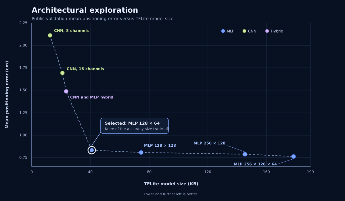
The larger MLPs continued to reduce positioning error, but the improvement became progressively smaller as the model size increased. The deepest 256 → 128 → 64 MLP achieved the lowest mean error of 0.762 cm, but its TFLite model was 178 KB and its Pico inference took approximately 75 ms.
The CNNs were smaller and faster, but their mean errors remained between 1.49 cm and 2.11 cm. One plausible reason is that the nine inputs are not interchangeable image pixels. Each channel represents a fixed LED with its own physical position and intensity response. Convolution assumes that a useful local pattern can be shared across different parts of the grid, which may not hold for these location-specific RSS fingerprints. The 3 × 3 input is also very small, leaving little room for a CNN to build a useful hierarchy of spatial features. In comparison, an MLP can directly learn relationships between every LED channel.
The 128 → 64 MLP sat near the knee of the Pareto front. Its final run reached 0.833 cm mean error with a 41 KB model and 16.54 ms Pico inference time. The deepest MLP improved the mean error by only 0.071 cm, while requiring approximately 4.35 times more model storage and 4.5 times more inference time. For a microcontroller deployment, that was not a worthwhile trade-off, so I selected the float 128 → 64 MLP for the final submission.
Final Task 1 result
Mean positioning error is the average Euclidean distance between the predicted and true receiver positions, measured in centimetres. Lower values indicate better positioning accuracy.
| Metric | Baseline | Final model |
|---|---|---|
| Architecture | 9 → 32 → 32 → 2 |
9 → 128 → 64 → 2 |
| Mean positioning error | 5.86 cm | 0.833 cm |
| TFLite model size | 8.7 KB | 41.0 KB |
| Pico inference latency | 2.13 ms | 16.54 ms |
The final model reduced the mean positioning error by approximately 85.8%. It was larger and slower than the baseline, but accuracy carried the highest weight in Task 1, making this a trade-off I was comfortable with.
Task 2: Repairing noisy RSS on the Pico
Task 1 produced an accurate model when the RSS measurements were clean. Task 2 removed that assumption. The input now contained dropouts, ghost readings, and attenuation, but the weights of Model A had to remain unchanged. This meant the problem had to be solved entirely through deterministic preprocessing on the Pico.
Understanding the raw measurements
The raw data showed three important corruption modes:
- Dropouts: An LED expected to be visible produced a value of zero.
- Ghost readings: A normally dark channel produced a small nonzero value.
- Multiplicative noise: Visible channels were attenuated or otherwise distorted.
Approximately 5.5 of the nine channels changed in a typical raw sample. When these measurements were passed directly to the frozen Task 1 model, the mean positioning error increased to 15.14 cm. Repeated measurements from the same location were also scattered throughout the data stream, which made simple grouped median filtering impractical on the Pico.
Building the on-device denoiser
Instead of asking Model A to interpret measurements that no longer resembled its training data, I used a physical model of the lighting environment to estimate what the clean RSS fingerprint should have looked like. The repaired measurements could then be passed to the same frozen model used in Task 1.
The complete pipeline was:
I first fitted a separate light-propagation model for each of the nine LEDs using the clean training fingerprints, based on Lambert’s cosine law. The hackathon formulation extended the basic cosine law with the LED’s Lambertian order, distance-dependent propagation loss, the receiver incidence angle, and a field-of-view cutoff. Together, these terms provided a continuous approximation of the RSS value expected from every LED at a given receiver position.
At startup, the Pico used these models to generate a quantized fingerprint table over the room with a grid spacing of 4 cm. The fingerprints were stored as uint16 values, keeping the table at approximately 86 KB of RAM.
For every raw RSS vector, the firmware searched this table for the closest physical fingerprint. It used a capped absolute-residual cost so that a dropout or unusually large channel error could not dominate the match. Once the closest fingerprint was found:
- Expected illuminated channels that had dropped to zero were imputed.
- Large channel outliers were replaced with their physics-based estimates.
- The remaining measurements were blended with the expected values.
The corrected nine-channel vector was then standardized and passed to Model A without changing any of its trained weights.
Final Task 2 result
Across the first 5,000 public raw-validation samples:
| Metric | Raw input | Physics-based repair |
|---|---|---|
| Mean positioning error | 15.14 cm | 7.85 cm |
| p95 positioning error | 60.02 cm | 20.34 cm |
The denoiser reduced the mean positioning error by approximately 48%. Because retraining Model A on the noisy measurements was not allowed, the improvement had to come from preprocessing. The physics-based repair moved each corrupted RSS vector closer to the clean input distribution expected by the frozen model.
Task 3: Learning from sparse measurements with physics
Task 2 used physics to repair corrupted measurements before inference. Task 3 used the same general idea for a different purpose: creating the dense training data that the provided measurements could not supply.
This time, the model received RSS values from all 36 LEDs in the 6 × 6 configuration. However, the dataset contained only 703 training fingerprints and 78 public validation fingerprints, with measurements spaced 8 cm apart. The hidden evaluation used a much denser 1 cm resolution. Training directly on the 703 available points risked teaching the network the sparse sampling grid rather than the continuous relationship between light intensity and position.
Turning sparse measurements into dense training data
I fitted a separate Lambertian light-propagation model for each of the 36 LEDs using the sparse training fingerprints. Together, these models provided a continuous approximation of the complete 36-channel RSS fingerprint at any position in the room.
I then sampled 250,000 random continuous positions and generated their fingerprints using the fitted physics models. To make these synthetic measurements less idealized, I added Gaussian sensor noise and applied randomized detection thresholds that turned sufficiently weak LED values into zero.
The real 703 fingerprints were repeated 20 times and mixed into the synthetic dataset. This anchored the network to actual measurements instead of allowing the approximated physics model to dominate the training data. The resulting dataset contained 264,060 samples.
Designing Model B
The expanded dataset was used to train a compact MLP:
Input (36) → 64 → 64 → Output (2)All 36 RSS channels were standardized independently before training. The model was trained for 60 epochs using Adam, MSE loss, shuffled mini-batches, and a cosine learning-rate schedule.
Although Model B received four times as many input channels as the Task 1 model, I kept its hidden layers smaller. The dense synthetic coverage carried much of the generalization burden, allowing the deployed network to remain compact.
Final Task 3 result
I exported both a float model and an int8 candidate and evaluated them on the 78 real sparse validation fingerprints:
| Variant | TFLite size | Mean error | p95 error |
|---|---|---|---|
| Float | 29,332 bytes | 0.828 cm | 1.488 cm |
| Int8 candidate | 12,960 bytes | 1.042 cm | 1.952 cm |
Quantization reduced the model size by approximately 56%, but increased the mean positioning error by 0.214 cm. Since positioning accuracy carried the greatest weight in Task 3, I retained the non-quantized float model for the final submission.
Task 4: Adapting to LED aging online
Task 4 returned to the nine-LED configuration and the frozen Model A from Task 1. This time, however, the brightness of each LED decreased as the installation aged. The evaluation stream was divided into deployment episodes, with every episode representing a later operating age. Rare flicker events and additive noise were also applied to individual measurements.
The aging simulation assigned each LED its own decay rate. Its brightness at operating time t was modelled as:
Here, T90,j is the time at which LED j retains 90% of its original brightness. Because every LED had a different T90, the nine channels did not fade by the same amount. Model A had been trained on the original brightness distribution, so this uneven decay created an increasing mismatch between its training data and the measurements it received.
Tracking one gain per LED
The central idea was to estimate this brightness loss online. The Pico maintained one gain value for each LED, with all nine gains initialized to one. Before inference, every incoming RSS value was divided by its current gain estimate to approximate the original unaged brightness.
The corrected fingerprint was then robustly matched against the same Lambertian reference table introduced in Task 2. This produced an expected clean fingerprint for the estimated position. The relationship between the observed and expected intensity provided a new estimate of how much each LED had faded.
The complete loop was:
For a nonzero channel with a sufficiently strong expected value, the firmware calculated an observed-to-expected ratio and updated the gain using a bounded exponential moving average:
The bounds prevented one unusual measurement from producing an unrealistic gain, while the update rate of 0.06 allowed the estimate to follow gradual aging without reacting too strongly to individual samples. After an episode change, the calibration generally settled around the new brightness level within roughly 50 samples.
The physics fingerprint also helped with per-sample corruption. Unexpected zeros were treated as flicker and replaced when the corresponding LED was expected to be visible. Large deviations were replaced with their physics-based estimates, while reasonable measurements were blended gently toward the expected values.
All of this adaptation happened in the input-calibration layer. The weights of Model A were never changed.
Final Task 4 result
The complete pipeline was evaluated over all 4,685 public validation samples using ten aging episodes and seed 123:
| Metric | Without adaptation | Online calibration |
|---|---|---|
| Mean positioning error | 7.555 cm | 1.369 cm |
| p95 positioning error | 17.008 cm | 2.921 cm |
Without adaptation, the mean error increased from 2.539 cm in the youngest episode to 11.915 cm in the oldest. With online calibration, the per-episode mean remained between 1.143 cm and 1.678 cm.
The online calibration reduced the overall mean positioning error by approximately 82%. Task 4 combined the robust physics matching from Task 2 with a small amount of state that continuously adjusted the input signals as the LEDs aged, while keeping the original positioning model frozen.
Conclusion
Looking back, the biggest lesson from the hackathon was that a better edge AI system is not defined by the AI model alone, but by the complete system built around it. Task 1 benefited from better preprocessing, training, and architecture choices. Tasks 2 and 4 kept that model frozen and handled changing input conditions around it, while Task 3 used the physics of visible light to create the dense training data that was otherwise missing.
Across all four tasks, the most effective approach was to combine a compact neural network with knowledge of the physical system. The neural networks learned the relationship between RSS fingerprints and position, while the Lambertian model helped repair corrupted measurements, interpolate sparse data, and adapt to aging LEDs. This combination allowed the final solutions to remain practical for the Raspberry Pi Pico without treating the model as the answer to every problem.
Together, these optimizations earned our team second place in the hackathon. More than the final ranking, the rewarding part was seeing the complete pipeline move from data analysis and model training to firmware running on a microcontroller.